XLOOKUP Function
The Excel XLOOKUP function is the successor to the VLOOKUP and HLOOKUP functions
Original Idea
The basic 3-parameter version of the XLOOKUP function presents almost a one-to-one implementation of the vector form of LOOKUP function with the removed requirement for the one-row or one-column lookup_array (lookup_vector) to be sorted as shown below:

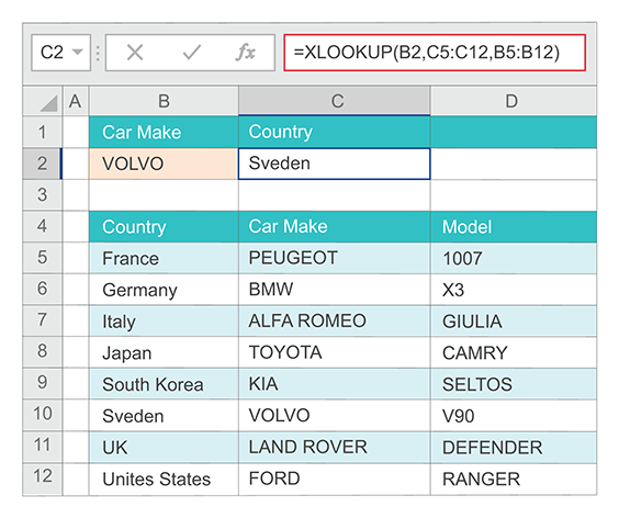
This example uses a XLOOKUP to look up a car make, then returns its model. It includes lookup_value ("VOLVO"), lookup_array (range C5:C12), and return_array (range D5:D12) arguments. The basic 3-parameter XLOOKUP defaults to an exact match and does not require the lookup_array to be sorted.
Search in Any Column or Row
The lookup_array plays the role of the first column or row of a table array and the return_array is used instead of a table array column or row, which contains the return value. Subsequently, users are no longer forced to perform a search in the first column for the VLOOKUP or in the first row for the HLOOKUP function. Thus, the return_array column can be to the left of the lookup_array column and the return_array row can be above the lookup_array row as shown below:

This example uses a XLOOKUP to look up a car make, then returns its country.
Return Array with Multiple Items
The removal of the Google Sheets LOOKUP function requirement for the return_array to appear as a single column or a single row allowed XLOOKUP to not only supersede the VLOOKUP and HLOOKUP functions, but also to operate as the MATCH and INDEX functions in conjunction as shown below:

This example is looking up movie information based on its budget. Unlike VLOOKUP, XLOOKUP is able to return an array with multiple items, which allows a single formula to return both genre and title from cells B8:C8. In this example the lookup_array (range D5:D12) is to the right of the return_array (range B5:C12) represented by two adjacent columns "Genre" and "Title".
Not Found Message
The advanced version of the XLOOKUP functions added three additional optional parameters: if_not_found, match_mode, and search_mode. This allowed the XLOOKUP function to achieve extraordinary flexibility. The if_not_found parameter supplies the value or text to replace the #N/A when a search fails to find a match as shown in the example below:

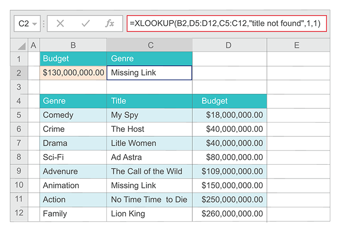
In this example we added the if_not_found parameter to the formula in the previous example.
Match Mode
The match_mode parameter increased the accuracy of the XLOOKUP search criterion specification as compared to the VLOOKUP, HLOOKUP, and MATCH functions. For example, a wildcard characters search is clearly specified in XLOOKUP by the match_mode parameter equal to a wildcard match (2), so a wildcard characters search is initiated by this setting and not by the presence of wildcard characters in the lookup_value. The XLOOKUP match_mode parameter defaults to the exact match (0), which is not the case for the VLOOKUP, HLOOKUP, and MATCH functions defaulting to an approximate match. This should be considered a step forward.
Search Mode
The search_mode parameter defines a search method that will be used by the XLOOKUP functions. There are 16 possible combinations of the match_mode and search_mode parameter values. Only four of them do not require sorting lookup_array elements. For example, when the match_mode parameter equals to the exact match (0) and the search_mode parameter equals to the reverse search (-1), a search will be performed from right to left when the lookup_array is a single row, or from bottom to top when it is a single column. The search_mode parameter in this case defines a search direction, which may be critical when the lookup_array has duplicate elements.
The below example uses both the match_mode and search_mode arguments:

This example looks in column D for the budget entered in cell B2, and finds a matching title in column C. It sets the if_not_found argument to return a "Title not found" text if nothing is found. The match_mode argument is set to 1, which means the function will look for an exact match, and if it can't find one, it will return the next larger item. Finally, the search_mode argument is set to 1, which means the function will search from the first item to the last.
Nested XLOOKUP
A nested XLOOKUP function can be used to perform both a vertical and horizontal match as shown below:.

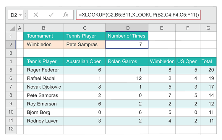
In this example a nested XLOOKUP function will first look for Wimbledon Grand Slam tournament in row 4, then look for the player named Pete Sampras in column C, and return the value at the intersection of the two. This is similar to using the INDEX and MATCH functions in conjunction.


